

Statistical Fashions vs. Entrance-Line Staff: Who Is aware of Greatest The way to Spend Opioid Settlement Money?
[ad_1]
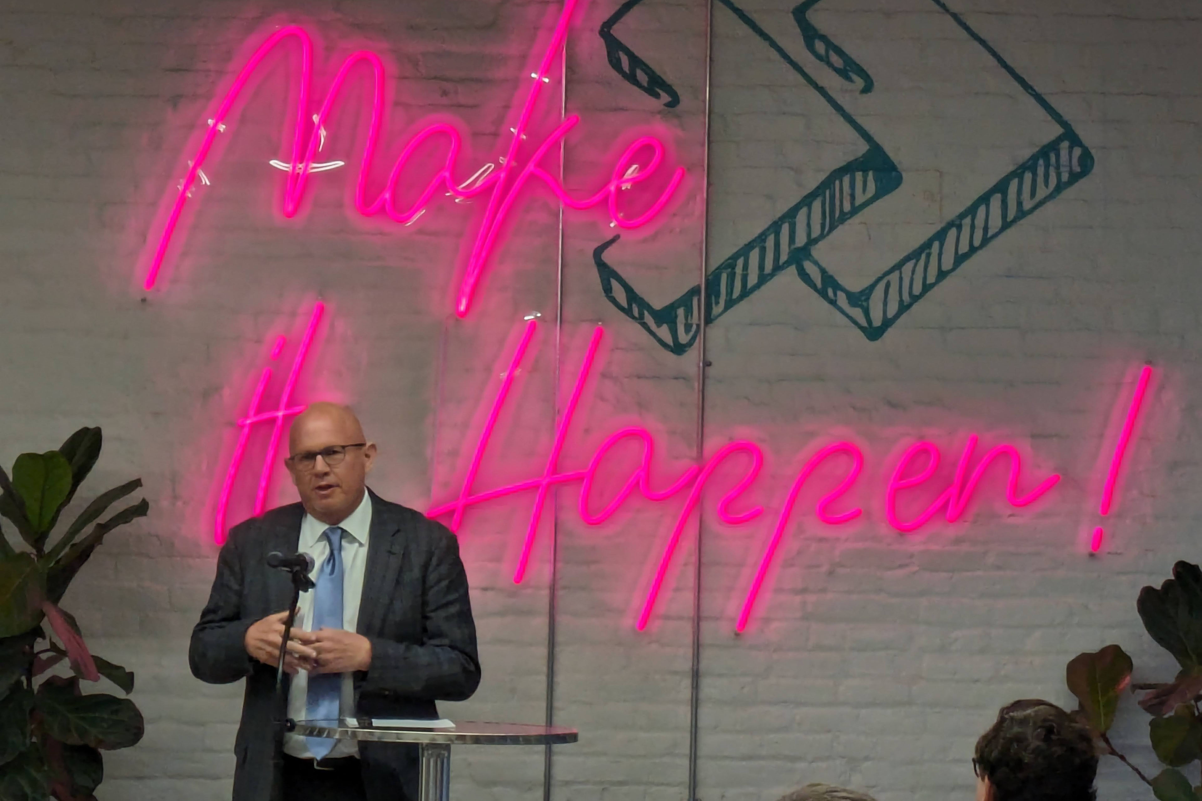
MOBILE, Ala. — In this Gulf Coast city, addiction medicine doctor Stephen Loyd announced at a January event what he called “a game-changer” for state and local governments spending billions of dollars in opioid settlement funds.
The money, which comes from companies accused of aggressively marketing and distributing prescription painkillers, is meant to tackle the addiction crisis.
But “how do you know that the money you’re spending is going to get you the result that you need?” asked Loyd, who was once hooked on prescription opioids himself and has become a nationally known figure since Michael Keaton played a character partially based on him in the Hulu series “Dopesick.”
Loyd provided an answer: Use statistical modeling and artificial intelligence to simulate the opioid crisis, predict which programs will save the most lives, and help local officials decide the best use of settlement dollars.
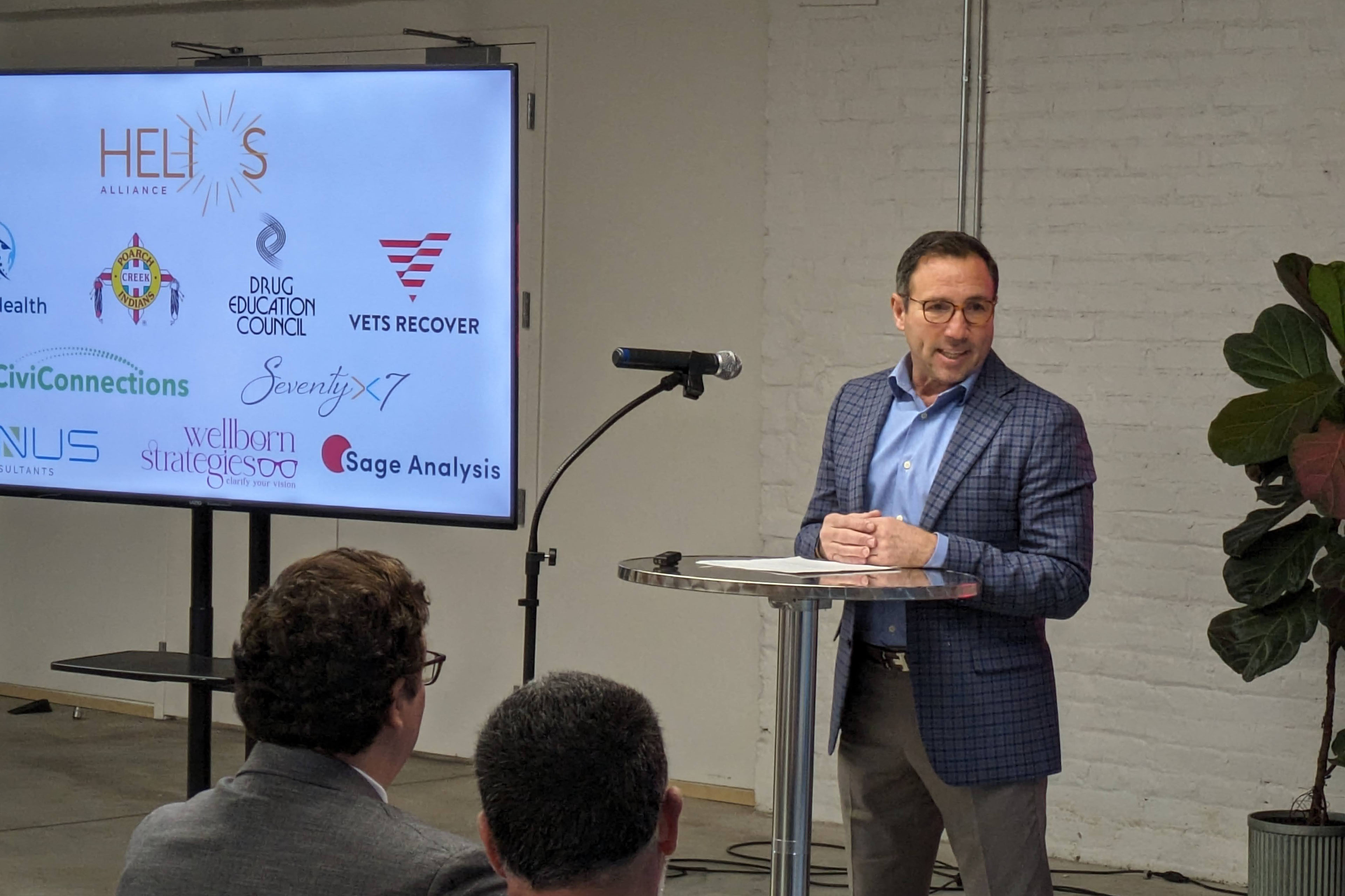
Loyd serves as the unpaid co-chair of the Helios Alliance, a group that hosted the event and is seeking $1.5 million to create such a simulation for Alabama.
The state is set to receive more than $500 million from opioid settlements over nearly two decades. It announced $8.5 million in grants to various community groups in early February.
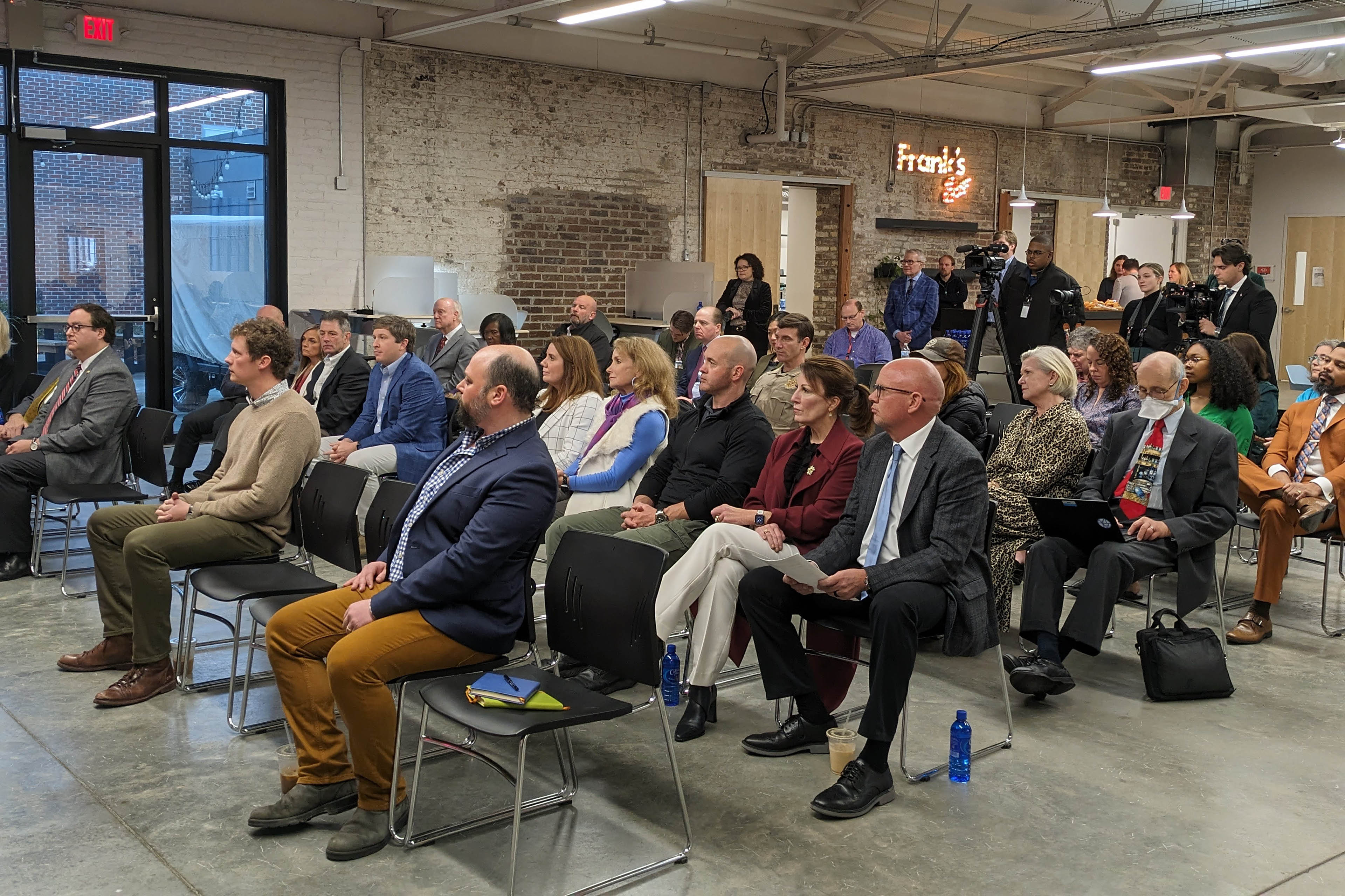
Loyd’s audience that gray January morning included big players in Mobile, many of whom have known one another since their school days: the speaker pro tempore of Alabama’s legislature, representatives from the city and the local sheriff’s office, leaders from the nearby Poarch Band of Creek Indians, and dozens of addiction treatment providers and advocates for preventing youth addiction.
Many of them were excited by the proposal, saying this type of data and statistics-driven approach could reduce personal and political biases and ensure settlement dollars are directed efficiently over the next decade.
But some advocates and treatment providers say they don’t need a simulation to tell them where the needs are. They see it daily, when they try — and often fail — to get people medications, housing, and other basic services. They worry allocating $1.5 million for Helios prioritizes Big Tech promises for future success while shortchanging the urgent needs of people on the front lines today.
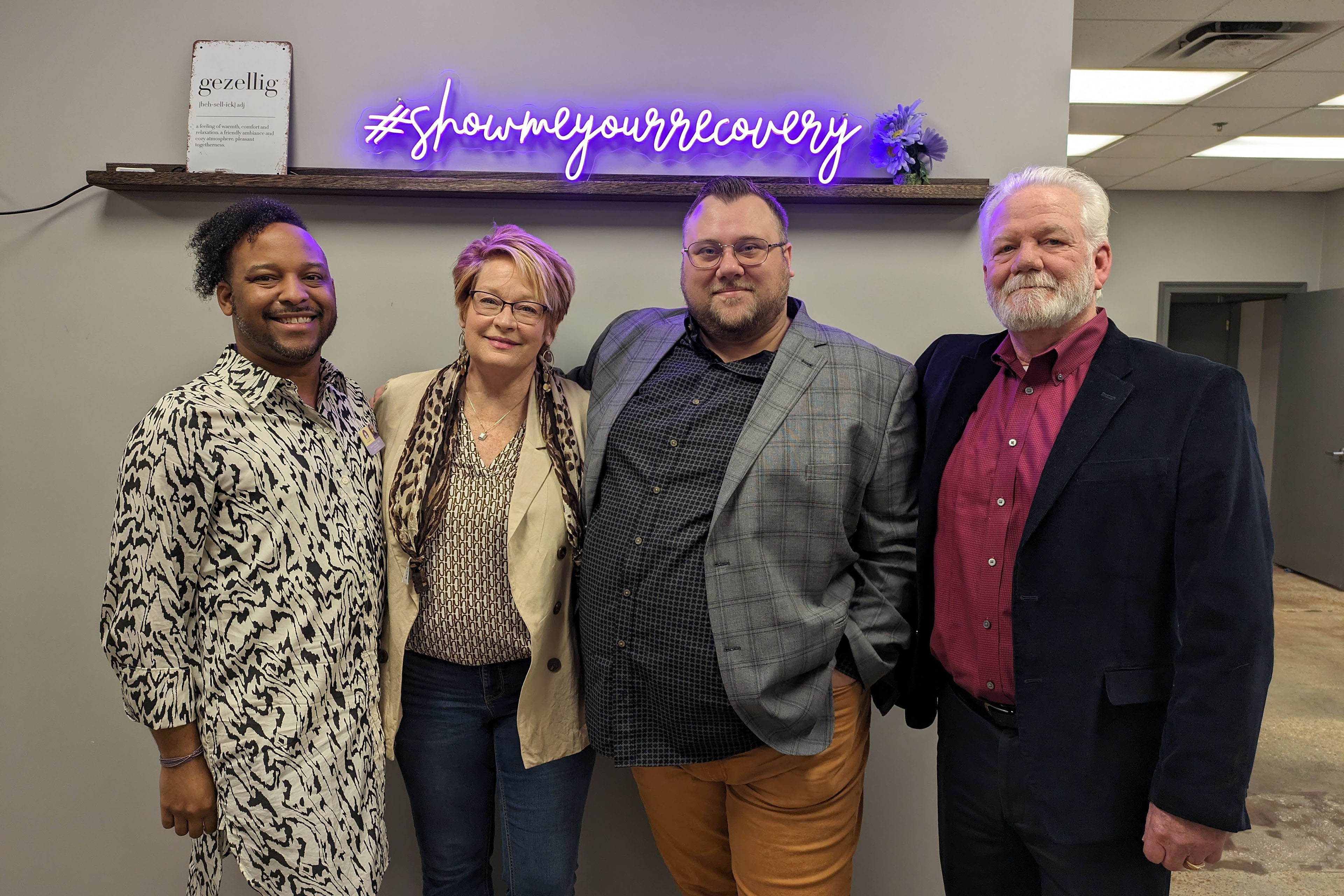
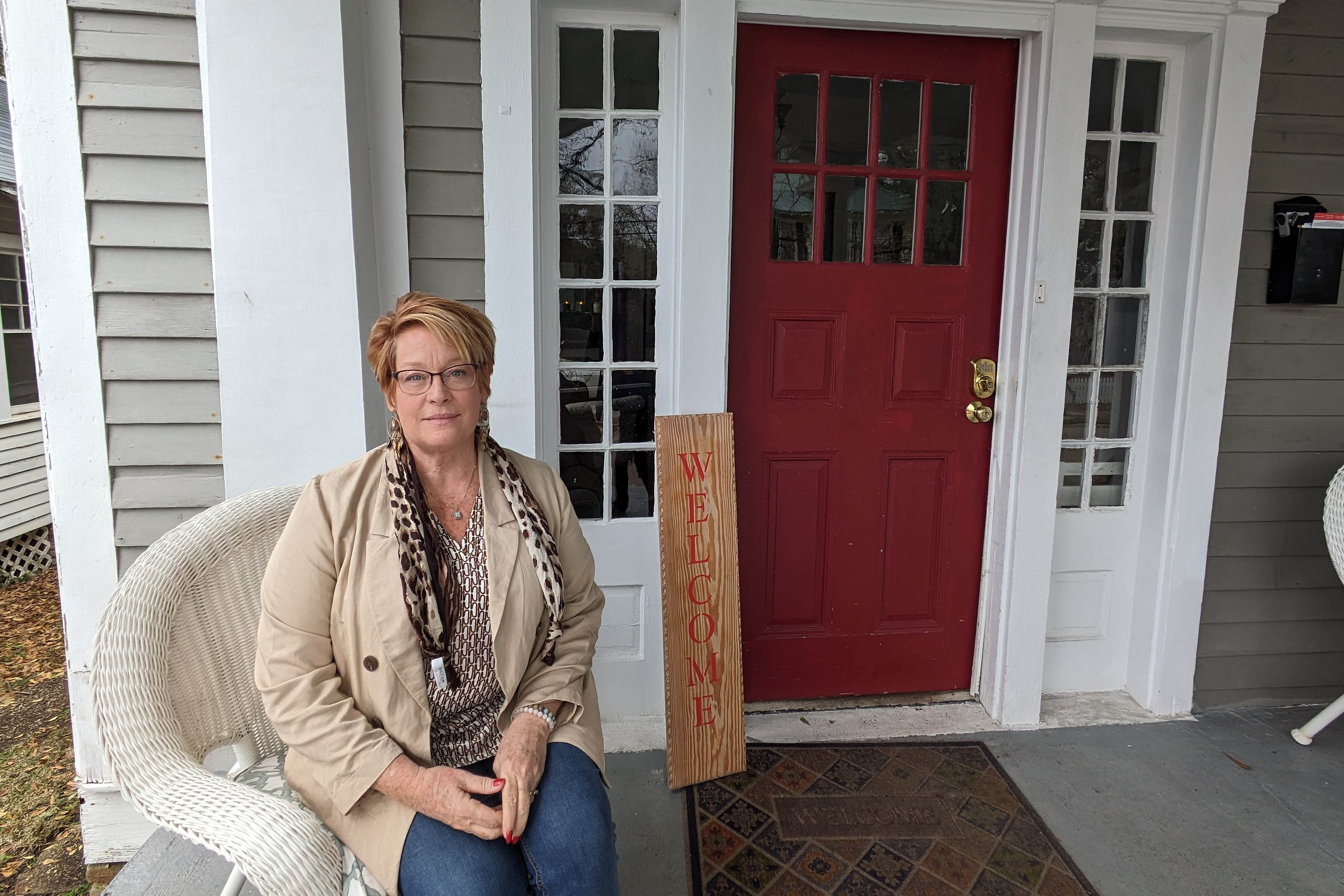
“Data does not save lives. Numbers on a computer do not save lives,” said Lisa Teggart, who is in recovery and runs two sober living homes in Mobile. “I’m a person in the trenches,” she said after attending the Helios event. “We don’t have a clean-needle program. We don’t have enough treatment. … And it’s like, when is the money going to get to them?”
The debate over whether to invest in technology or boots on the ground is likely to reverberate widely, as the Helios Alliance is in discussions to build similar models for other states, including West Virginia and Tennessee, where Loyd lives and leads the Opioid Abatement Council.
New Predictive Promise?
The Helios Alliance comprises nine nonprofit and for-profit organizations, with missions ranging from addiction treatment and mathematical modeling to artificial intelligence and marketing. As of mid-February, the alliance had received $750,000 to build its model for Alabama.
The largest chunk — $500,000 — came from the Poarch Band of Creek Indians, whose tribal council voted unanimously to spend most of its opioid settlement dollars to date on the Helios initiative. A state agency chipped in an additional $250,000. Ten Alabama cities and some private foundations are considering investing as well.
Stephen McNair, director of external affairs for Mobile, said the city has an obligation to use its settlement funds “in a way that is going to do the most good.” He hopes Helios will indicate how to do that, “instead of simply guessing.”
Rayford Etherton, a former attorney and consultant from Mobile who created the Helios Alliance, said he is confident his team can “predict the likely success or failure of programs before a dollar is spent.”
The Helios website features a similarly bold tagline: “Going Beyond Results to Predict Them.”
To do this, the alliance uses system dynamics, a mathematical modeling technique developed at the Massachusetts Institute of Technology in the 1950s. The Helios model takes in local and national data about addiction services and the drug supply. Then it simulates the effects different policies or spending decisions can have on overdose deaths and addiction rates. New data can be added regularly and new simulations run anytime. The alliance uses that information to produce reports and recommendations.
Etherton said it can help officials compare the impact of various approaches and identify unintended consequences. For example, would it save more lives to invest in housing or treatment? Will increasing police seizures of fentanyl decrease the number of people using it or will people switch to different substances?
And yet, Etherton cautioned, the model is “not a crystal ball.” Data is often incomplete, and the real world can throw curveballs.
Another limitation is that while Helios can suggest general strategies that might be most fruitful, it typically can’t predict, for instance, which of two rehab centers will be more effective. That decision would ultimately come down to individuals in charge of awarding contracts.
Mathematical Models vs. On-the-Ground Experts
To some people, what Helios is proposing sounds similar to a cheaper approach that 39 states — including Alabama — already have in place: opioid settlement councils that provide insights on how to best use the money. These are groups of people with expertise ranging from addiction medicine and law enforcement to social services and personal experience using drugs.
Even in places without formal councils, treatment providers and recovery advocates say they can perform a similar function. Half a dozen advocates in Mobile told KFF Health News the city’s top need is low-cost housing for people who want to stop using drugs.
“I wonder how much the results” from the Helios model “are going to look like what people on the ground doing this work have been saying for years,” said Chance Shaw, director of prevention for AIDS Alabama South and a person in recovery from opioid use disorder.
But Loyd, the co-chair of the Helios board, sees the simulation platform as augmenting the work of opioid settlement councils, like the one he leads in Tennessee.
Members of his council have been trying to decide how much money to invest in prevention efforts versus treatment, “but we just kind of look at it, and we guessed,” he said — the way it’s been done for decades. “I want to know specifically where to put the money and what I can expect from outcomes.”
Jagpreet Chhatwal, an expert in mathematical modeling who directs the Institute for Technology Assessment at Massachusetts General Hospital, said models can reduce the risk of individual biases and blind spots shaping decisions.
If the inputs and assumptions used to build the model are transparent, there’s an opportunity to instill greater trust in the distribution of this money, said Chhatwal, who is not affiliated with Helios. Yet if the model is proprietary — as Helios’ marketing materials suggest its product will be — that could erode public trust, he said.
Etherton, of the Helios Alliance, told KFF Health News, “Everything we do will be available publicly for anyone who wants to look at it.”
Urgent Needs vs. Long-Term Goals
Helios’ pitch sounds simple: a small upfront cost to ensure sound future decision-making. “Spend 5% so you get the biggest impact with the other 95%,” Etherton said.
To some people working in treatment and recovery, however, the upfront cost represents not just dollars, but opportunities lost for immediate help, be it someone who couldn’t find an open bed or get a ride to the pharmacy.
“The urgency of being able to address those individual needs is vital,” said Pamela Sagness, executive director of the North Dakota Behavioral Health Division.
Her department recently awarded $7 million in opioid settlement funds to programs that provide mental health and addiction treatment, housing, and syringe service programs because that’s what residents have been demanding, she said. An additional $52 million in grant requests — including an application from the Helios Alliance — went unfunded.
Back in Mobile, advocates say they see the need for investment in direct services daily. More than 1,000 people visit the office of the nonprofit People Engaged in Recovery each month for recovery meetings, social events, and help connecting to social services. Yet the facility can’t afford to stock naloxone, a medication that can rapidly reverse overdoses.
At the two recovery homes that Mobile resident Teggart runs, people can live in a drug-free space at a low cost. She manages 18 beds but said there’s enough demand to fill 100.
Hannah Seale felt lucky to land one of those spots after leaving Mobile County jail last November.
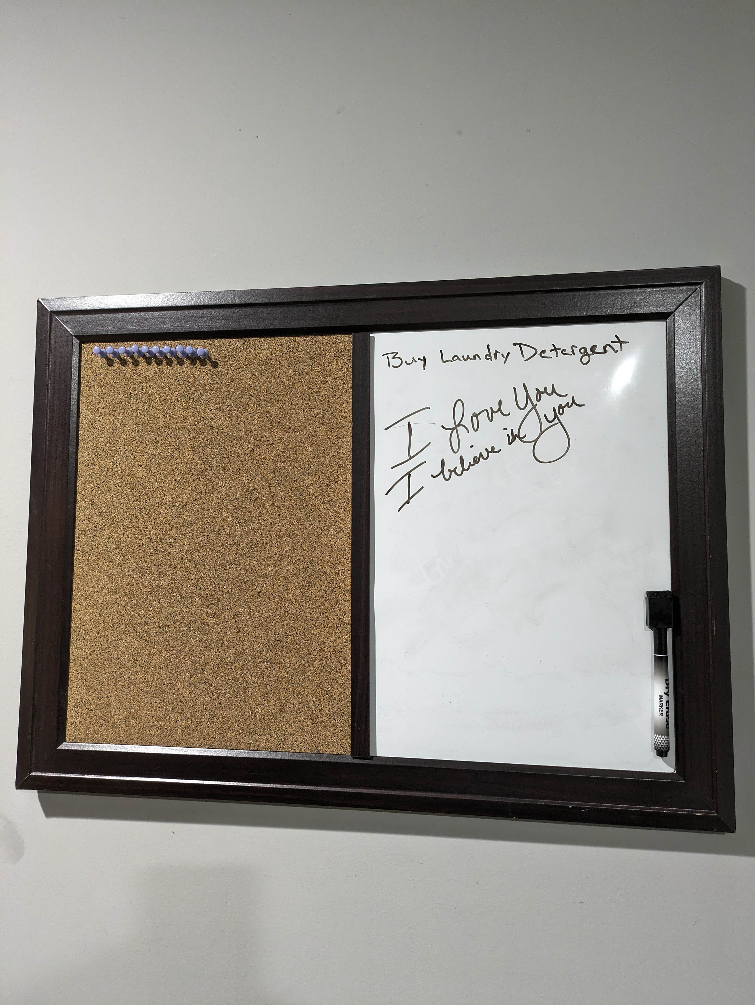
“All I had with me was one bag of clothes and some laundry detergent and one pair of shoes,” Seale said.
Since arriving, she’s gotten her driver’s license, applied for food stamps, and attended intensive treatment. In late January, she was working two jobs and reconnecting with her 4- and 7-year-old daughters.
After 17 years of drug use, the recovery home “is the one that’s worked for me,” she said.
Comments are closed.